NRT data#
import time

import matplotlib.pyplot as plt
import pandas as pd

import uscrn
Recent hourly data#
With uscrn.get_nrt_data(), we can load recent data (near-real-time) from USCRN
by specifying the period we want and from which dataset.
Here, we request the 6 most recent files.
now = pd.Timestamp.now("UTC")
print(now)

df = uscrn.get_nrt_data(
    (-6, None),
    "hourly",
    n_jobs=2,
)
Show code cell output
2025-04-16 14:03:03.075960+00:00
Discovering files...
  Looking for files in these years
  - 2025
Found 6 file(s) to load
https://www.ncei.noaa.gov/pub/data/uscrn/products/hourly02/updates/2025/CRN60H0203-202504160800.txt
...
https://www.ncei.noaa.gov/pub/data/uscrn/products/hourly02/updates/2025/CRN60H0203-202504161300.txt
Reading files...
[Parallel(n_jobs=2)]: Using backend LokyBackend with 2 concurrent workers.
[Parallel(n_jobs=2)]: Done 1 tasks | elapsed: 1.0s
[Parallel(n_jobs=2)]: Done   4 out of   6 | elapsed:    1.5s remaining:    0.8s
[Parallel(n_jobs=2)]: Done   6 out of   6 | elapsed:    1.7s finished
df
| wban | utc_time | lst_time | crx_vn | longitude | latitude | t_calc | t_hr_avg | t_max | t_min | ... | soil_moisture_5 | soil_moisture_10 | soil_moisture_20 | soil_moisture_50 | soil_moisture_100 | soil_temp_5 | soil_temp_10 | soil_temp_20 | soil_temp_50 | soil_temp_100 | |
|---|---|---|---|---|---|---|---|---|---|---|---|---|---|---|---|---|---|---|---|---|---|
| 0 | 03047 | 2025-04-16 07:00:00 | 2025-04-16 01:00:00 | 2.622 | -102.809998 | 31.620001 | 19.5 | 19.799999 | 20.4 | 19.500000 | ... | 0.017 | 0.024 | 0.043 | 0.035 | 0.035 | 22.700001 | 22.200001 | 25.400000 | 24.700001 | 23.1 |
| 1 | 03048 | 2025-04-16 07:00:00 | 2025-04-16 00:00:00 | 2.622 | -106.889999 | 34.360001 | 16.5 | 16.700001 | 17.6 | 16.299999 | ... | 0.044 | 0.068 | 0.071 | 0.062 | 0.063 | 21.500000 | 23.600000 | 23.200001 | 20.299999 | 18.9 |
| 2 | 03054 | 2025-04-16 07:00:00 | 2025-04-16 01:00:00 | 2.622 | -102.769997 | 33.959999 | 9.8 | 10.100000 | 10.7 | 7.300000 | ... | 0.139 | 0.173 | 0.203 | 0.154 | 0.132 | 16.500000 | 18.200001 | 18.400000 | 17.600000 | 15.3 |
| 3 | 03055 | 2025-04-16 07:00:00 | 2025-04-16 01:00:00 | 2.622 | -101.589996 | 36.599998 | 9.0 | 9.400000 | 9.9 | 9.000000 | ... | 0.200 | 0.247 | 0.257 | 0.393 | 0.259 | 13.600000 | 14.300000 | 13.900000 | 13.300000 | 13.0 |
| 4 | 03060 | 2025-04-16 07:00:00 | 2025-04-16 00:00:00 | 2.622 | -107.690002 | 38.540001 | 5.7 | 6.000000 | 6.4 | 5.700000 | ... | 0.201 | 0.285 | 0.295 | 0.321 | 0.255 | 7.300000 | 7.900000 | 7.900000 | 5.900000 | 4.5 |
| ... | ... | ... | ... | ... | ... | ... | ... | ... | ... | ... | ... | ... | ... | ... | ... | ... | ... | ... | ... | ... | ... |
| 932 | 96405 | 2025-04-16 12:00:00 | 2025-04-16 03:00:00 | 2.514 | -145.350006 | 60.470001 | 3.3 | 3.300000 | 3.5 | 3.000000 | ... | NaN | NaN | NaN | NaN | NaN | NaN | NaN | NaN | NaN | NaN |
| 933 | 96406 | 2025-04-16 12:00:00 | 2025-04-16 03:00:00 | 2.515 | -154.130005 | 64.500000 | 0.5 | 0.100000 | 0.6 | -0.100000 | ... | NaN | NaN | NaN | NaN | NaN | NaN | NaN | NaN | NaN | NaN |
| 934 | 96407 | 2025-04-16 12:00:00 | 2025-04-16 03:00:00 | 2.515 | -159.000000 | 66.559998 | -6.6 | -7.300000 | -6.6 | -8.200000 | ... | NaN | NaN | NaN | NaN | NaN | NaN | NaN | NaN | NaN | NaN |
| 935 | 96408 | 2025-04-16 12:00:00 | 2025-04-16 03:00:00 | 2.515 | -150.869995 | 63.450001 | -1.8 | -1.700000 | -1.3 | -1.900000 | ... | NaN | NaN | NaN | NaN | NaN | NaN | NaN | NaN | NaN | NaN |
| 936 | 96409 | 2025-04-16 12:00:00 | 2025-04-16 03:00:00 | 2.514 | -149.399994 | 68.650002 | -10.2 | -10.500000 | -9.8 | -11.300000 | ... | NaN | NaN | NaN | NaN | NaN | NaN | NaN | NaN | NaN | NaN |
937 rows × 36 columns
Sometimes, a few sites can have times an hour earlier than the others.
See the notes in uscrn.get_nrt_data() for more details.
def func(x):
    nx = len(x)
    if nx == 0:
        return ""
    elif nx < 10:
        return sorted(x.unique())
    else:
        return f"..."

(
    df.utc_time
    .value_counts()
    .sort_index()
    .to_frame()
    .assign(
        wbans=df.groupby("utc_time")["wban"].apply(func),
    )
)
| count | wbans | |
|---|---|---|
| utc_time | ||
| 2025-04-16 07:00:00 | 157 | ... |
| 2025-04-16 08:00:00 | 156 | ... |
| 2025-04-16 09:00:00 | 156 | ... |
| 2025-04-16 10:00:00 | 156 | ... |
| 2025-04-16 11:00:00 | 156 | ... |
| 2025-04-16 12:00:00 | 156 | ... |
In these files, for example, site WBAN 13301 has data for multiple earlier days included.
https://www.ncei.noaa.gov/pub/data/uscrn/products/hourly02/updates/2024/CRN60H0203-202402212000.txt
https://www.ncei.noaa.gov/pub/data/uscrn/products/hourly02/updates/2024/CRN60H0203-202402222000.txt
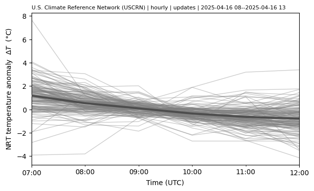
Plot temperature change time series#
fig, ax = plt.subplots(figsize=(7, 4))

df_ = df.copy()

tmax = df_.utc_time.max()
df_ = df_[df_.utc_time.between(tmax - pd.Timedelta("7h"), tmax)]

df_["utc_time_mid"] = df_["utc_time"] + pd.Timedelta("30min")
df_["t_hr_avg_k"] = df_["t_hr_avg"].add(273.15)
df_["dt_hr_avg"] = df_["t_hr_avg_k"].sub(df_.groupby("wban")["t_hr_avg_k"].transform("mean"))

df_[["utc_time", "dt_hr_avg"]].groupby("utc_time").mean().plot(
    color="0.3",
    linewidth=3,
    zorder=10,
    legend=False,
    ax=ax,
)

df_.groupby("wban").plot(
    x="utc_time",
    y="dt_hr_avg",
    color="0.5",
    linewidth=1,
    alpha=0.4,
    legend=False,
    xlabel="Time (UTC)",
    ylabel="NRT temperature anomaly  $\Delta T$  (°C)",
    ax=ax,
)

ax.set_title(df.attrs["title"], loc="left", size=8);
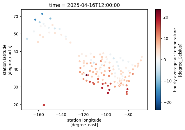
Plot current temperature#
fig, ax = plt.subplots(figsize=(7, 4.5))

ds = uscrn.to_xarray(df)

ds.isel(time=-1).plot.scatter(x="longitude", y="latitude", hue="t_hr_avg", ax=ax);
Specific period of hourly data#
Date selection works by file, not by the data inside the file.
In general, the data are an hour behind the file date/time.
See the notes in uscrn.get_nrt_data() for more details.
def get_nrt_hourly_period(period):
    a, b = period
    ap1 = pd.to_datetime(a) + pd.Timedelta(hours=1)
    bp1 = pd.to_datetime(b) + pd.Timedelta(hours=1)

    df = uscrn.get_nrt_data((ap1, bp1))

    time.sleep(0.5)  # for prints
    in_period = df.utc_time.between(a, b)
    print(
        f"Got {in_period.sum()}/{len(df)} ({in_period.sum() / len(df):.1%}) records "
        f"in desired period {a} to {b}"
    )
    outside = df.loc[~in_period, "utc_time"].value_counts()
    print(
        "Outside counts:",
        ", ".join(f"{time:%Y-%m-%d %H} ({count})" for time, count in outside.items())
    )

    dupe = df.duplicated(["wban", "utc_time"], keep=False)
    print(f"Got {dupe.sum()} ({dupe.sum() / len(df):.1%}) duplicates")

    return (
        df[in_period]
        .drop_duplicates(["wban", "utc_time"], keep="last")
        .reset_index(drop=True)
    )


df = get_nrt_hourly_period(("2024-02-09 16", "2024-02-09 20"))
Show code cell output
/home/docs/checkouts/readthedocs.org/user_builds/uscrn/envs/v0.2.0/lib/python3.11/site-packages/uscrn/data.py:773: UserWarning: Timestamp 2024-02-09 17:00:00 has no timezone, assuming UTC.
  warnings.warn(f"Timestamp {ts} has no timezone, assuming UTC.")
/home/docs/checkouts/readthedocs.org/user_builds/uscrn/envs/v0.2.0/lib/python3.11/site-packages/uscrn/data.py:773: UserWarning: Timestamp 2024-02-09 21:00:00 has no timezone, assuming UTC.
  warnings.warn(f"Timestamp {ts} has no timezone, assuming UTC.")
Discovering files...
  Looking for files in these years
  - 2024
Found 5 file(s) to load
https://www.ncei.noaa.gov/pub/data/uscrn/products/hourly02/updates/2024/CRN60H0203-202402091700.txt
...
https://www.ncei.noaa.gov/pub/data/uscrn/products/hourly02/updates/2024/CRN60H0203-202402092100.txt
Reading files...
[Parallel(n_jobs=2)]: Using backend LokyBackend with 2 concurrent workers.
[Parallel(n_jobs=2)]: Done   1 tasks      | elapsed:    0.2s
[Parallel(n_jobs=2)]: Batch computation too fast (0.17067646980285645s.) Setting batch_size=2.
[Parallel(n_jobs=2)]: Done   3 out of   5 | elapsed:    0.3s remaining:    0.2s
[Parallel(n_jobs=2)]: Done   5 out of   5 | elapsed:    0.5s finished
Got 769/771 (99.7%) records in desired period 2024-02-09 16 to 2024-02-09 20
Outside counts: 2024-02-09 15 (2)
Got 6 (0.8%) duplicates
df
| wban | utc_time | lst_time | crx_vn | longitude | latitude | t_calc | t_hr_avg | t_max | t_min | ... | soil_moisture_5 | soil_moisture_10 | soil_moisture_20 | soil_moisture_50 | soil_moisture_100 | soil_temp_5 | soil_temp_10 | soil_temp_20 | soil_temp_50 | soil_temp_100 | |
|---|---|---|---|---|---|---|---|---|---|---|---|---|---|---|---|---|---|---|---|---|---|
| 0 | 03047 | 2024-02-09 16:00:00 | 2024-02-09 10:00:00 | 2.622 | -102.809998 | 31.620001 | 11.300000 | 10.0 | 11.300000 | 8.300000 | ... | 0.048 | 0.038 | 0.056 | 0.045 | 0.035 | 9.3 | 9.1 | 9.5 | 12.1 | 13.3 |
| 1 | 03048 | 2024-02-09 16:00:00 | 2024-02-09 09:00:00 | 2.622 | -106.889999 | 34.360001 | 3.000000 | 2.3 | 3.100000 | 0.900000 | ... | 0.101 | 0.140 | 0.109 | 0.056 | 0.057 | 3.1 | 4.4 | 6.2 | 8.2 | 9.2 |
| 2 | 03054 | 2024-02-09 16:00:00 | 2024-02-09 10:00:00 | 2.622 | -102.769997 | 33.959999 | 6.700000 | 6.5 | 6.700000 | 5.900000 | ... | 0.132 | 0.160 | 0.164 | 0.105 | 0.125 | 5.0 | 5.8 | 6.9 | 9.0 | 10.3 |
| 3 | 03055 | 2024-02-09 16:00:00 | 2024-02-09 10:00:00 | 2.622 | -101.589996 | 36.599998 | 8.700000 | 6.7 | 8.700000 | 3.900000 | ... | 0.250 | 0.306 | 0.324 | 0.412 | 0.217 | 4.5 | 5.0 | 5.6 | 6.4 | 6.6 |
| 4 | 03060 | 2024-02-09 16:00:00 | 2024-02-09 09:00:00 | 2.622 | -107.690002 | 38.540001 | -7.400000 | -8.4 | -7.400000 | -10.400000 | ... | NaN | NaN | NaN | 0.173 | 0.152 | -0.3 | -0.3 | -0.1 | 0.7 | 2.0 |
| ... | ... | ... | ... | ... | ... | ... | ... | ... | ... | ... | ... | ... | ... | ... | ... | ... | ... | ... | ... | ... | ... |
| 761 | 94996 | 2024-02-09 20:00:00 | 2024-02-09 14:00:00 | 2.622 | -96.849998 | 40.700001 | 8.200000 | 7.8 | 8.400000 | 7.000000 | ... | 0.290 | 0.330 | 0.287 | 0.260 | 0.322 | 5.1 | 4.4 | 4.8 | 5.2 | 5.5 |
| 762 | 96404 | 2024-02-09 20:00:00 | 2024-02-09 11:00:00 | 2.514 | -141.210007 | 62.740002 | -21.700001 | -22.9 | -21.700001 | -24.200001 | ... | NaN | NaN | NaN | NaN | NaN | NaN | NaN | NaN | NaN | NaN |
| 763 | 96405 | 2024-02-09 20:00:00 | 2024-02-09 11:00:00 | 2.514 | -145.350006 | 60.470001 | 3.000000 | 2.9 | 3.200000 | 2.600000 | ... | NaN | NaN | NaN | NaN | NaN | NaN | NaN | NaN | NaN | NaN |
| 764 | 96407 | 2024-02-09 20:00:00 | 2024-02-09 11:00:00 | 2.515 | -159.000000 | 66.559998 | -9.700000 | -9.3 | -8.700000 | -11.100000 | ... | NaN | NaN | NaN | NaN | NaN | NaN | NaN | NaN | NaN | NaN |
| 765 | 96409 | 2024-02-09 20:00:00 | 2024-02-09 11:00:00 | 2.514 | -149.399994 | 68.650002 | -10.800000 | -9.6 | -8.000000 | -11.100000 | ... | NaN | NaN | NaN | NaN | NaN | NaN | NaN | NaN | NaN | NaN |
766 rows × 36 columns
Recent daily data#
Here, we load the most recent daily data file.
df = uscrn.get_nrt_data(-1, "daily")
Show code cell output
Discovering files...
  Looking for files in these years
  - 2025
Found 1 file(s) to load
https://www.ncei.noaa.gov/pub/data/uscrn/products/daily01/updates/2025/CRND0103-202504152359.txt
Reading files...
[Parallel(n_jobs=1)]: Done   1 tasks      | elapsed:    3.3s
[Parallel(n_jobs=1)]: Done   1 tasks      | elapsed:    3.3s
df
| wban | lst_date | crx_vn | longitude | latitude | t_daily_max | t_daily_min | t_daily_mean | t_daily_avg | p_daily_calc | ... | soil_moisture_5_daily | soil_moisture_10_daily | soil_moisture_20_daily | soil_moisture_50_daily | soil_moisture_100_daily | soil_temp_5_daily | soil_temp_10_daily | soil_temp_20_daily | soil_temp_50_daily | soil_temp_100_daily | |
|---|---|---|---|---|---|---|---|---|---|---|---|---|---|---|---|---|---|---|---|---|---|
| 0 | 03047 | 2025-04-15 | 2.622 | -102.809998 | 31.620001 | 26.600000 | 13.3 | 20.000000 | 19.9 | 0.0 | ... | 0.018 | 0.024 | 0.044 | 0.035 | 0.035 | 25.700001 | 26.0 | 25.400000 | 24.4 | 23.200001 |
| 1 | 03048 | 2025-04-15 | 2.622 | -106.889999 | 34.360001 | 28.100000 | 10.5 | 19.299999 | 19.4 | 0.0 | ... | 0.046 | 0.068 | 0.070 | 0.063 | 0.063 | 25.000000 | 23.4 | 21.900000 | 19.9 | 18.799999 |
| 2 | 03054 | 2025-04-15 | 2.622 | -102.769997 | 33.959999 | 22.400000 | 6.0 | 14.200000 | 14.4 | 0.0 | ... | 0.142 | 0.175 | 0.204 | 0.154 | 0.132 | 18.900000 | 18.1 | 17.700001 | 17.4 | 15.200000 |
| 3 | 03055 | 2025-04-15 | 2.622 | -101.589996 | 36.599998 | 22.500000 | 1.7 | 12.100000 | 11.8 | 0.0 | ... | 0.201 | 0.247 | 0.257 | 0.396 | 0.258 | 13.900000 | 14.1 | 13.500000 | 13.3 | 12.900000 |
| 4 | 03060 | 2025-04-15 | 2.622 | -107.690002 | 38.540001 | 16.200001 | 2.3 | 9.300000 | 8.0 | 0.0 | ... | 0.204 | 0.286 | 0.295 | 0.324 | 0.256 | 8.500000 | 8.0 | 7.400000 | 5.9 | 4.400000 |
| ... | ... | ... | ... | ... | ... | ... | ... | ... | ... | ... | ... | ... | ... | ... | ... | ... | ... | ... | ... | ... | ... |
| 151 | 96405 | 2025-04-15 | 2.514 | -145.350006 | 60.470001 | 8.100000 | -5.4 | 1.300000 | 2.3 | 2.0 | ... | NaN | NaN | NaN | NaN | NaN | NaN | NaN | NaN | NaN | NaN |
| 152 | 96406 | 2025-04-15 | 2.515 | -154.130005 | 64.500000 | 6.400000 | -4.1 | 1.100000 | 1.9 | 0.0 | ... | NaN | NaN | NaN | NaN | NaN | NaN | NaN | NaN | NaN | NaN |
| 153 | 96407 | 2025-04-15 | 2.515 | -159.000000 | 66.559998 | -6.900000 | -19.1 | -13.000000 | -11.6 | 0.5 | ... | NaN | NaN | NaN | NaN | NaN | NaN | NaN | NaN | NaN | NaN |
| 154 | 96408 | 2025-04-15 | 2.515 | -150.869995 | 63.450001 | 4.700000 | -1.6 | 1.600000 | 1.4 | 0.0 | ... | NaN | NaN | NaN | NaN | NaN | NaN | NaN | NaN | NaN | NaN |
| 155 | 96409 | 2025-04-15 | 2.514 | -149.399994 | 68.650002 | -4.800000 | -22.9 | -13.800000 | -14.0 | 0.0 | ... | NaN | NaN | NaN | NaN | NaN | NaN | NaN | NaN | NaN | NaN |
156 rows × 28 columns
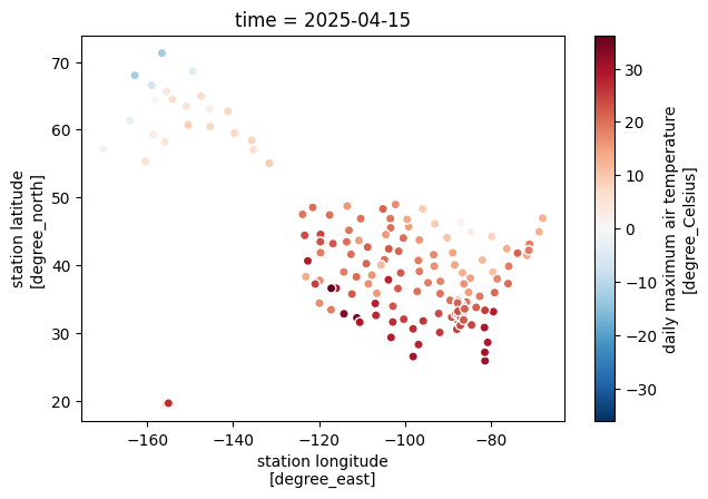
fig, ax = plt.subplots(figsize=(7, 4.5))

ds = uscrn.to_xarray(df).squeeze()

ds.plot.scatter(x="longitude", y="latitude", hue="t_daily_max", ax=ax);